1  Data Collection and Overview

1.0.1 Population

The population data is constructed using IBGE’s yearly municipal population estimates. We download and manually pre-process the data into one consolidated excel file: /input/population/population_BR_municipio_year.xlsx. We impute 2010 my averaging 2009 and 2011 population figures per municipality. We re-create the 7-digit municipality identifier by combining 2-digit UF and five-digit municipality codes; adding leading zeroes to the five-digit codes wherever necessary. We merge telecommunications and population data by year and (7-digit) municipio codes.

Code

pop 

Estimated Population at the Municipality - Year level

1.0.2 Telecoms

The telecommunications data was collected from an Anatel API which grants access to open telecommunications data at the year-month-municipality-provider-transmission-technology-speed level. The data indicates the number of accesses for each group. Table (telecoms_data_sample?) depicts an example of the clean source data. Table (year_month_mun?) is the collapsed data-set at the year-month-municipality level.

Code

microdata_sample

Clean ANATEL Micro-data

First 10,000 observations

Code

microdata_output

Output data-set: Number of accesses per year-month-municipality

2007

Code

# 
# muni <- read_municipality()
# 
# plotting_microdata_output <- microdata_output %>% copy() %>%  .[year==2007] %>% .[month==12] %>% 
#   dplyr::left_join(muni, ., by = c("code_muni" = "municipio"))
# 
# breaks_qt <- classIntervals(c(min(plotting_microdata_output$total_accesses_per_pop) - .0000001, plotting_microdata_output$total_accesses_per_pop), n = 10, style = "quantile")
# 
# plotting_microdata_output <- mutate(plotting_microdata_output, total_accesses_per_pop_cat = cut(total_accesses_per_pop, breaks_qt$brks)) 

plotting_microdata_output %>% .[which(plotting_microdata_output$year==2007), ] %>% 
  ggplot(data=.) +
  geom_sf(aes(fill=total_accesses_per_pop_cat), color= NA, size=.15) +
    labs(subtitle="Total Number of Telecom Contracts per Population, 2007", size=8) +
      scale_fill_brewer(palette = "RdYlBu") + 
    # scale_fill_distiller(palette = "Blues", name="Ratio") +
    theme_minimal() + 
  theme(legend.title = element_blank())

Notice that all three panels: 2007, 2012, and 2019 are directly comparable.

Total Number of Telecom Contracts per Population (2007, December)

2012

Code

plotting_microdata_output %>% .[which(plotting_microdata_output$year==2012), ] %>% 
  ggplot(data=.) +
  geom_sf(aes(fill=total_accesses_per_pop_cat), color= NA, size=.15) +
    labs(subtitle="Total Number of Telecom Contracts per Population, 2012", size=8) +
      scale_fill_brewer(palette = "RdYlBu") + 
    # scale_fill_distiller(palette = "Blues", name="Ratio") +
    theme_minimal() + 
  theme(legend.title = element_blank())

Notice that all three panels: 2007, 2012, and 2019 are directly comparable.

Total Number of Telecom Contracts per Population (2012, December)

2019

Code

# muni <- read_municipality()
# 
# plotting_microdata_output <- microdata_output %>% copy() %>%  .[year==2019] %>% .[month==12] %>% 
#   dplyr::left_join(muni, ., by = c("code_muni" = "municipio"))
# 
# breaks_qt <- classIntervals(c(min(plotting_microdata_output$total_accesses_per_pop) - .0000001, plotting_microdata_output$total_accesses_per_pop), n = 10, style = "quantile")
# 
# plotting_microdata_output <- mutate(plotting_microdata_output, total_accesses_per_pop_cat = cut(total_accesses_per_pop, breaks_qt$brks)) 


plotting_microdata_output %>% .[which(plotting_microdata_output$year==2019), ] %>% 
  ggplot(data=.) +
  geom_sf(aes(fill=total_accesses_per_pop_cat), color= NA, size=.15) +
    labs(subtitle="Total Number of Telecom Contracts per Population, 2019", size=8) +
      scale_fill_brewer(palette = "RdYlBu") + 
    # scale_fill_distiller(palette = "Blues", name="Ratio") +
    theme_minimal() + 
  theme(legend.title = element_blank())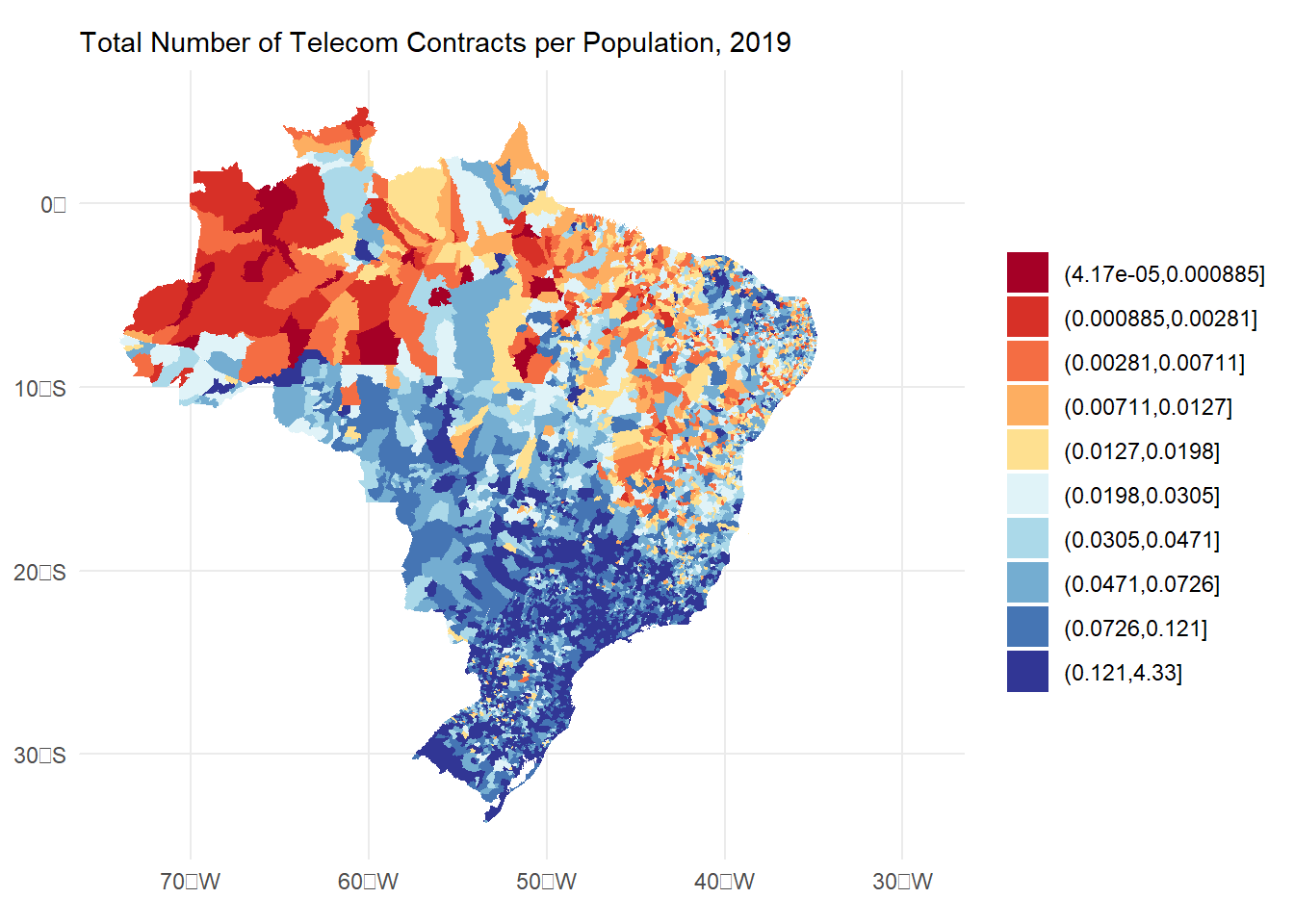

Notice that all three panels: 2007, 2012, and 2019 are directly comparable.

Total Number of Telecom Contracts per Population (2019, December)

1.1 What are the relevant categories we aggregate accross from the full data?

We aggregate accross provider, transmission, technology and speed. The following histograms depict the number of observations in the full data broken down by each of these categories.

Year

Code

microdata_year %>% 
  .[order(year)] 

Observations per year

Providers

Code

microdata_provider %>% 
  .[, sum(N), provider_name] %>% 
  .[order(-V1)] %>% 
  rename(., Accesses = V1 )

Number of accesses per provider for the full panel

Technology

Code

microdata_tech_gen %>% 
  .[, sum(N), .(technology, generation)] %>% 
  .[order(-V1)] %>% 
  rename(., Accesses = V1 )

Number of accesses per technology for the full panel

Generation

Code

microdata_tech_gen %>% 
  .[, sum(N), generation] %>% 
  .[order(-V1)] %>% 
  rename(., Accesses = V1 )

Number of accesses per generation for the full panel

Transmission

Code

microdata_transmission %>% 
  .[, sum(N), transmission] %>% 
  .[order(-V1)] %>% 
  rename(., Accesses = V1 )

Number of accesses per transmission type for the full panel

Speed

Code

microdata_speed %>% 
  .[, sum(N), speed] %>% 
  .[order(-V1)] %>% 
  rename(., Accesses = V1 ) 

Number of accesses per speed type for the full panel