2  First Attempt at Replication

This document was created for the week of April 24th 2023 with the goal of illustrating how I constructed a municipality-year level panel with the information required to replicate the main regressions from Corbi, Papaioannou, and Surico (2018). Secondly, the goal of the replication is to apply a novel political aspect to it. Therefore, the lower half of this section aims at understanding how politically affiliated firms are distributed in the main Political Connections data-set created with RAIS, TSE, RFB, CNE and PR data sources (Individual_RFB_CNE_RAIS_PR_yearly). Politically connected individuals are linked to parties through affiliation. For the purposes of the following output, politically connected firms have at least one owner with a formal political affiliation.

2.1 Paper Replication

2.1.1 Data Cleaning

For this initial stage, the objective is to quickly reconstruct the analysis from Corbi, Papaioannou, and Surico (2018). To that end, we use whatever is readily available first (namely data from the online Data Supplement), and supplement later on. The only exception is information from RAIS, which we replace with data from Individual_RFB_CNE_RAIS_PR_yearly instead.

2.1.1.1 Municipality - Year Panel

The code used to clean the data essentially processes the main Individual_RFB_CNE_RAIS_PR_yearly data-set (pc_data henceforth) and enriches it with information on firm-level owner affiliation status, constructed using the data-set itself. The result is an updated version of pc_data that is tabulated to create data-sets for plotting.

Municipality - Year Panel Steps

The municipality-year panel is constructed by taking the pc_data panel, indexed at the year-individual-firm level for owners and year-individual level for workers (with the worker’s highest paying job available) and simply:

1. Restricting pc_data to only workers
2. Tabulating the number of observations and average, non-missing pay per year-municipio-naturjur_cat; where municipio is the 5 digit municipality IBGE code and naturjur_cat distinguishes between private, public, non-profit and non-governmental organizations.
3. Finally, we merge the two tabulated data-sets on year-municipio-naturjur_cat.

2.1.1.2 IBGE Population

All the following population estimates mentioned are from IBGE. For the time being, we use estimates from the original paper whenever they are available (2002-2014). Additionally, we can supplement additional years (2015-2019) with data we cleaned from the IBGE website. Lastly, once we have advanced on other fronts, we will substitute all of these estimates with the clean version from the original FPM source data, as we can be certain those are point-in-time estimates and have not been revised later on. Given the sensitivity of the FPM cut-offs, it is crucial that we use the correct point in time data whenever it is available.

Estimates in the Paper

Given that the data supplement has IBGE population estimates up to 2014, for the purposes of the replication, we leverage the authors’ clean data for consistency. This leaves 2015-2019 to be supplemented.

Estimates we cleaned

We then take municipal population estimates from 2002-2019, sourced from files with yearly municipal population estimate from IBGE. We manually format them in excel. Data for 2010 is missing, so we impute population estimates by taking the simple average between 2009 and 2011 for all municipalities.

Estimates from FPM source

The next step is to extract the IBGE estimates from the original FPM data-sets, as the source material includes this information and is what is used to compute yearly transfers. This is preferred because any inconsistencies or revisions to the data have the potential to invalidate results from the analysis. E.g. Imagine there was an issue with IBGE figures for a specific municipality/year; since transfers are computed using that information, we should chose the incorrect point in time population estimates rather than the corrected figures.

2.1.1.3 Sample Restrictions

In order to replicate the original paper’s data set we include the same sample restrictions. Namely, we only include municipalities with 6,793 - 47,544 inhabitants according to IBGE and, for now, only consider 2002-2014.

2.1.1.4 Transfers

2.1.1.4.1 Data

We take the transfers data from the original data supplementation section, which runs from 1997 - 2014 and includes Federal Bolsa Familia, FPM and Finbra transfers data. The main data we are after is the FPM data though.

In addition to the data from the paper, we found the original FPM data-sets establishing the coefficients for each year. We have data-sets stretching between 2007-2019, though these must still be cleaned. For now, we use the data-set from the paper.

2.1.1.4.2 Actual vs Theoretical Transfers

When reading the paper, the methodology for constructing the transfers coefficients is a little messy. Here I explicitly go over each step so that there is no ambiguity.

1. Let \(FPM^t\) be the total yearly \(t\) FPM transfer pool the federal government allocates to states. Corbi, Papaioannou, and Surico (2018) highlight that by law, 22.5% of the total federal income and federal industrial tax revenue is dedicated to funding the FPM program. For simplicity, if we call \(\tau^t\) the total amount of yearly federal income and industrial tax revenue, \(FPM^t = (0.225)\tau^t\).

2. Let \(FPM^{k, t}\) be the FPM transfer allocated to state \(k\) in year \(t\). Each state has a fixed share \(s^{k, t}\) of the overall yearly \(FPM^t\) revenue pool, such that \(s^{k, t}*FPM^t = FPM^{k, t}\). Table (tab-fpm_state_allocation_coeff_91?) presents each state’s fixed percentage and sourced from Table 1, Appendix A from Corbi, Papaioannou, and Surico (2018). Notice that the values sum to 100.001 (%).

Code

fpm_state_coeff <- fread("data/fpm_state_allocation_coeff_91.csv") %>% 
  .[order(uf_name)]

3. Let \(FPM_i^{k,t}\) be the amount of resources allocated to municipality \(i\) in state \(k\) and year \(t\).

Since 2008, all municipalities have been required by law to follow the straightforward allocation equation: \(FPM_i^{k,t} = FPM_{k,t}\frac{\lambda^t_i}{\Sigma_{i \in k}\lambda^t_i}\); where \(\lambda^t_i\) is the yearly municipal FPM coefficient and \(\Sigma_{i \in k}\lambda^t_i\) is the state-wide aggregation of all its municipal coefficients.

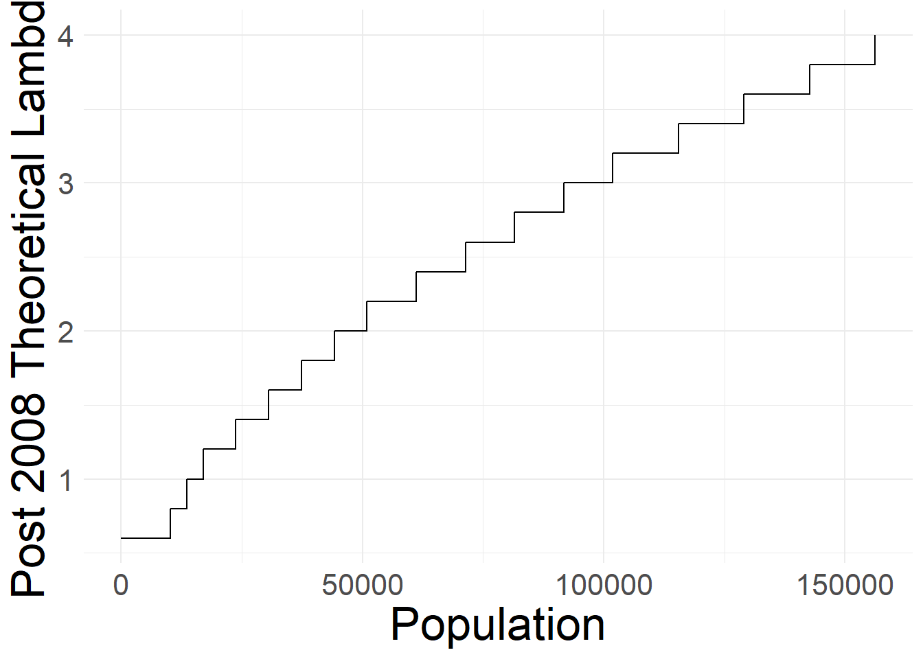
The \(\lambda^t_i\) coefficient increases discretely with previous year’s IBGE municipal population estimate \(pop^{t-1}_{i}\) and is the center piece for this project. Below, we also describe the alternate \(\tilde{\lambda}^t_i\), which takes special cases into account, prior to 2008. See table (tab-fpm_lambda_coeff_min_popest?) for a visualization of how population cut-offs map onto both the standard and alternate \(\lambda^t_i\) and \(\tilde{\lambda}^t_i\) theoretical coefficients.

Code

fread("data/fpm_lambda_coeff_min_popest.csv") %>% 
  ggplot(., aes(x=min_popest, y = lambda, label = lambda)) + 
    # geom_label_repel(size=4) +
    geom_step() +
    ylab("Post 2008 Theoretical Lambda") +
    xlab("Population") +
    theme_minimal() +
    theme(
      axis.title = element_text(size=25),
      legend.title = element_text(size=20),
      legend.position = "bottom",
      text = element_text(size=20)
    )

FPM Lambda Coefficient over Polulation

Code

  filename <- "images/fpm_lambda_coeff_min_popest.png"
  ggsave(plot = last_plot(), filename = filename, width = 16,height = 9, scale = 1)

Prior to 2008, some municipalities (usually the ones which came from municipality splits) were granted exceptions by the courts.

Therefore, prior to 2008, \(FPM_i^{k,t}\) has two concurrent definitions, depending on whether municipality \(i\) was legally afforded a benefit or not.

To keep things straightforward, we therefore define \(FPM_i^{k,t}\) generally, for all years, as:

\[ FPM_i^{k,t} = FPM_{k,t}\frac{\tilde{\lambda}^t_i}{\Sigma_{i \in k}\tilde{\lambda}^t_i} \]

where,

\[ \tilde{\lambda}^t_i =\begin{cases}\lambda^t_i & \text{if municipality } i \text{ DOES NOT have benefit} \\\alpha^t\lambda^t_i + (1-\alpha^t)\lambda^{97}_i & \text{if municipality } i \text{ DOES have benefit}\end{cases} \]

and

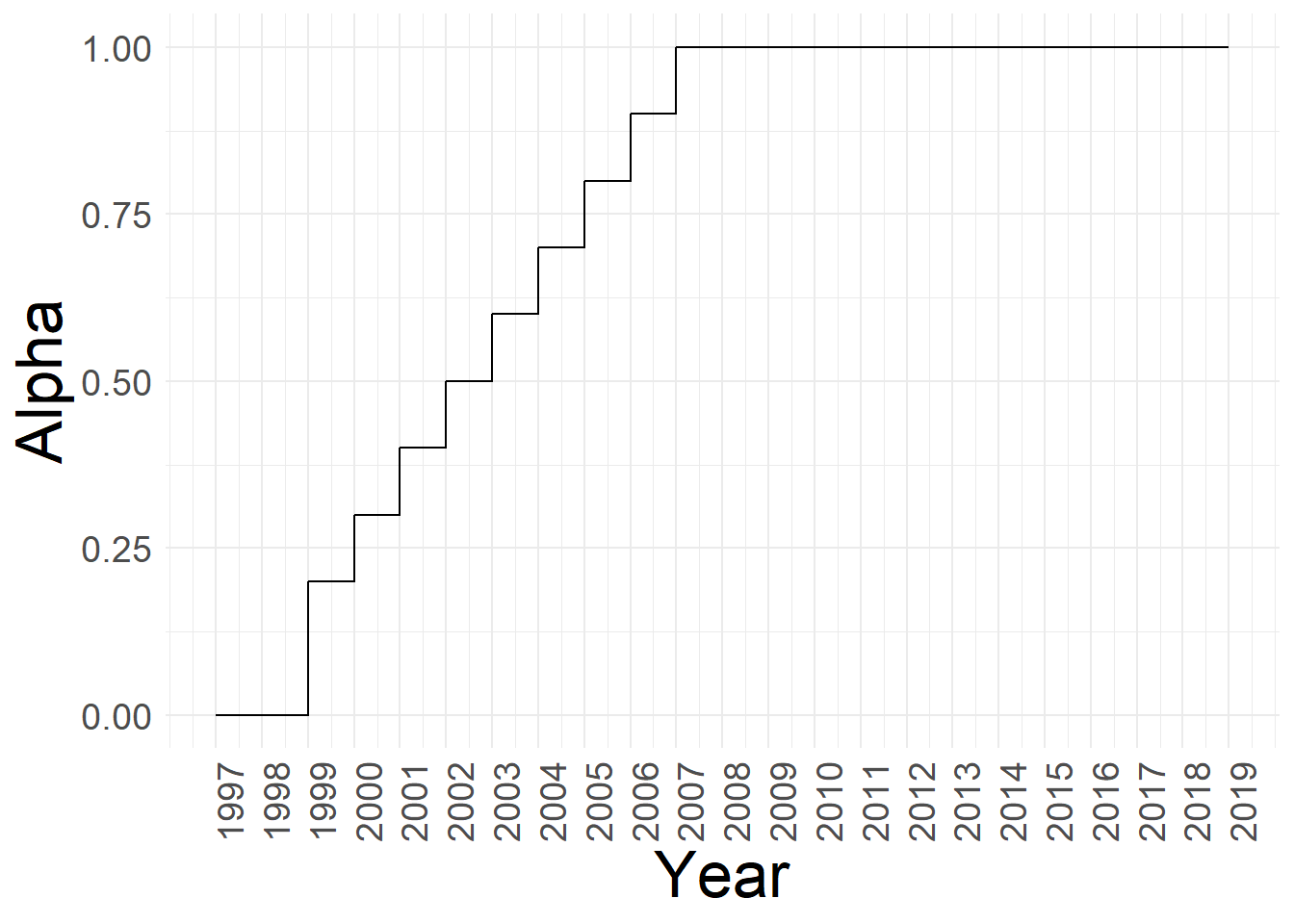
\[ \alpha^t =\begin{cases} 0 0.2 + (t - 1999)*0.1 & \text{if } t < 2008 \\1 & \text{if } t \geq 2008\end{cases} \]

That is, year \(t\) municipality \(i\) \(FPM^{k,t}_i\) is the share of the state \(k\)’s \(FPM^{k,t}\) transfer budget, where the share is computed as the fraction of the adjusted coefficient \(\hat{\lambda}^t_i\) over the sum of all of the municipalities’ adjusted coefficient \(\Sigma_{i \in k}\tilde\lambda^t_i\); where the adjustment is year and municipality contingent.

2.1.1.5 RED FLAGS 🚩

2.1.1.5.1 Constructing \(\alpha^t\)

In the documentation, \(\alpha^t\) is referred to as “redutor” or reducer. The documentation tells us that we ought to follow a simple rule to construct and apply it. When looking at how the original paper encodes it, they do not follow what is prescribed. See the box bellow for further details.

Potential Coding ERROR in original paper

Although Corbi, Papaioannou, and Surico (2018) presents a formula for computing \(\alpha^t\), either the simple formula or their code is incorrect. I use the formula from the paper to construct the \(\alpha^t\) ‘reductor’ variable.

Code

fread("data/fpm_alpha_redutor.csv") %>% 
  ggplot(., aes(x=year, y=alphat)) + 
  geom_step() +
    ylab("Alpha") +
    xlab("Year") +
    theme_minimal() + 
  scale_x_continuous(breaks = c(1997:2019)) + 
    theme(
      axis.title = element_text(size=25),
      legend.title = element_text(size=20),
      legend.position = "bottom",
      text = element_text(size=18),
      axis.text.x = element_text(angle=90)
    )

Code

  filename <- "images/fpm_alpha_redutor.png"
  ggsave(plot = last_plot(), filename = filename, width = 16,height = 9, scale = 1)

Code

knitr::include_graphics("images/redutor_formula.png")

Image taken from Regional Transfer Multiplier, Appendix A

Theoretical alpha computation perscribed in Appendix A

Code

knitr::include_graphics("images/redutor_code.png")

Code taken from data supplement from Regional Transfer Multiplier, Appendix A. This line of code creates the redutor, which is the pseudonym for the alpha parameter both in the code and the official FPM documentation.

Alpha computation in the “master.do” file

2.1.1.6 Constructing \(\hat{\lambda}^t_i\) and \(FPM^{k,t}_i\) more broadly

For some reason, Corbi, Papaioannou, and Surico (2018) construct their estimates in an extremely convoluted fashion, which does not make sense to me given the paper’s clear definition of how to compute the theoretical values are to be calculated. Below we include an image of this.

Code

knitr::include_graphics("images/replication_code_odd_construction_highlight.png")

Code taken from data supplement from Regional Transfer Multiplier, Appendix A. The hihglighted line of code creates the \(\hat{FPM}^{k,t}_{i}\) variable. This methodology is inconsisten with what is presented in the paper.

Inconsistent \(\hat{FPM}\) construction

2.1.1.7 Overcoming Red Flags

2.1.1.8 Clear identification of preferencially-treated municipalities

The central issue is that in their data, they do not identify which municipalities are subject to preferential treatment explicitly. This is limiting because the final allocations are supposedly based off of the ratio of a municipality’s adjusted coefficient over the sum of all municipal adjusted coefficients in the state-year. Therefore, without properly identifying which municipalities were assigned adjusted-FPM coefficients, there is no clear way of identifying the true FPM for all municipalities in the sample. This is quite a concerning issue.

The solution is that there is ample PDF documentation on which municipalities received subsidies. We should therefore read in these PDFs and construct a clean data-set with the full information from the time of allocation.

2.2 Identifying Municipalities with Fiscal Benefits

There is ample documentation (in PDF format) and data online which specify the municipalities which receive benefits, the specific benefit they receive and the prescribed \(\tilde{^\lambda}^{k,t}_{i}\) used for each municipality in each year. Thus far, it seems that there is only one benefit which is systematically applied, but it is never the less good to know that the documentation makes explicit comments on this issue.

We leverage the documentation found in the official TCU webpage that includes all of the documentation for the FPM transfers.

Data on FPM transfers can be found in .xls format for years following and including 2007. Data prior to 2007 is included in PDF format. We read in and clean these tables. Below, we will (eventually) include an example data-set.

2.2.0.1 Double-down on clarity and review all rules

Additionally, given that there appear to be multiple obvious short-falls with this article’s code, we cannot rule out additional hidden ones.

Hence forth, I suggest we be very clear on definitions and define what is needed for our paper.

First, by actual FPM transfers, we refer to the actual \(FPM^{k,t}_{i}\) received by each municipality. Second, by prescribed FPM transfer, we refer to the amount suggested in the yearly TCU spreadsheets. Prescribed FPM transfers are published in percentages of the state-year \(FPM_{k,t}\) budget, which is itself a fixed share of the total \(FPM_{t}\) federal pie. Lastly, by theoretical FPM transfer we refer to the FPM transfers delineated above.

THE LAST STEP TO CREATE THE DATA-SET IS IDENTIFING THESE MUNICIPALITIES.

This provides all of the pieces to reconstructing the initial part of the replication. The only missing step is to correctly identify which municipalities were affected by the benefit which ends in 2008.

:::

2.2.1 Output

2.2.1.1 Municipality - Year Data-set

The following data-set is indexed at the municipality level and presents, among other variables:

• log number of workers (both public and private),
• log total wages (in both public and private sector). This is the sum of all wages.
• population,
• actual transfers,
• implied transfers,
• population brackets used to compute the \(FPM_i^{k,t}\) transfers.

Given that we still need to merge in the pdf data identifier, implied transfer data for years prior to 2007 are not correct. Additionally, we still need to clean additional data from 2015 onwards.

Code

fread("data/fpm_mun_year_panel.csv")

Municipality-Year

This table presents a sample from the full municipality-year data-set. These are some of the best years in terms of data-coverage. The data leverages the transfer data-sets from the original paper and labor market outcomes from our political connections data-set, conditional on private and public sector employment. We drop statistics from non-governmental institutions, self-employed individuals and non-profits.

Code

fread("data/mun_year_panel.csv") %>% 
  .[, lapply(.SD, is.na), year] %>% 
  .[, lapply(.SD, sum), year] %>% 
  .[order(year)]

Municipality-Year Missing Data

This table presents the number of missing observations per year in the data-set. The data leverages the transfer data-sets from the original paper and labor market outcomes from our political connections data-set, conditional on private and public sector employment. We drop statistics from non-governmental institutions, self-employed individuals and non-profits.

2.3 Summary Statistics

2.3.1 Data Cleaning

Data for Figures

2.3.2 Workers and Wages

The municipality-year panel is constructed by taking the pc_data panel, indexed at the year-individual-firm level for owners and year-individual level for workers (with the worker’s highest paying job available) and simply:

1. Indicating that a firm is politically affiliated in a year if at least one owner is affiliated in that year.

2. Dropping owners from the panel such that it is indexed at the worker-year level and computing: the number of unique municipalities (municipio) and plants (plantid) associated with a firm (firmid) in a given year. We call these variables N_multi_municipal_firm and N_multi_plant_firm. when working on Colonnelli, Pinho Neto, and Teso (2022), plants were labelled as plants only they were in separate municipalities. Hence, we create two measures of plants to accommodate for the official RAIS and the municipal definitions.

3. We also combine the Blue Collar, White collar or Manager indcators into one variable to tabulate in the next step. Not all workers fall into these bins, so we keep observations from the un-matched missing category as well.

4. To construct the figures, we tabulate the data into two broad data-sets for each plant definition:

   1. First, we tabulate the number of observations from the worker-year data-set by year, N_multi_municipal_firm, firm_affiliated, worker_type.

   2. Second, we reduce the data-set to the firmid-year level, and tabulate the data by year, N_multi_plant_firm and firm_affiliated.

2.3.3 Figures

Code

# load data-sets to create figures 

  # MULTI PLANT -----
  N_multi_plant_firm_year_aff <-
  fread(file = "data/N_multi_plant_firm_year_aff.csv")

  # MULTI MUNICIPALITY  -----
  N_multi_municipal_firm_year_aff <- 
  fread(file ="data/N_multi_municipal_firm_year_aff.csv")

  # MULTI plant by worker type  -----s
  N_worker_type_I_multi_plant_firm_year_aff <-
  fread( "data/N_worker_type_I_multi_plant_firm_year_aff.csv")

  # MULTI MUNICIPALITY by worker type  -----
  N_worker_type_I_multi_municipal_firm_year_aff <-
  fread("data/N_worker_type_I_multi_municipal_firm_year_aff.csv")

2.3.4 Number and Share of Multi-Plant Firms over Time

CNPJ

Code

  item1_plant <- N_multi_plant_firm_year_aff %>%
    copy() %>%
    # indicate if multiplant firm
    .[, I_multi_plant_firm  := N_multi_plant_firm > 1] %>%
    .[, sum(N, na.rm=T), .(year, I_multi_plant_firm )] %>%
    .[, share := round(V1/sum(V1), digits = 3), year]

  item1_plant %>%
    ggplot(., aes(x = year, y = V1, color = I_multi_plant_firm, label = scales::percent(share, trim = F))) +
    geom_label_repel(size=4) +
    geom_point() +
    geom_line() +
    ylab("Count") +
    xlab("Year") +
    labs(color = "Multi-Plant firm") +
    scale_y_continuous(labels = scales::label_comma()) + 
    theme_minimal() +
    theme(
      axis.title = element_text(size=25),
      legend.title = element_text(size=20),
      legend.position = "bottom",
      text = element_text(size=20)
    )

  filename <- "images/N_and_share_multi_plant_firms.png"
  ggsave(plot = last_plot(), filename = filename, width = 16,height = 9, scale = 1)

We define a Multi-Plant Firm as having more than one plants, as defined by the last four digits in a firms CNPJ, excluding the last two verification digits. All firms have at least one plant by definition. The boxes in the graph indicate the yearly share of firms which are either multi-plant or not.

Share and Number of Firms that are Multi-Plants over Time

Municipal

Code

  item1_municipal <- N_multi_municipal_firm_year_aff %>%
    copy() %>%
    # indicate if multimunicipal firm
    .[, I_multi_municipal_firm  := N_multi_municipal_firm > 1] %>%
    .[, sum(N, na.rm=T), .(year, I_multi_municipal_firm )] %>%
    .[, share := round(V1/sum(V1), digits = 3), year]

  item1_municipal %>%
    ggplot(., aes(x = year, y = V1, color = I_multi_municipal_firm, label = scales::percent(share, trim = F))) +
    geom_label_repel(size=4) +
    geom_point() +
    geom_line() +
    scale_y_continuous(labels = scales::label_comma()) + 
    ylab("Count") +
    xlab("Year") +
    labs(color = "Multi-Municipal firm") +
    scale_y_continuous(labels = scales::label_comma()) + 
    theme_minimal() +
    theme(
      axis.title = element_text(size=25),
      legend.title = element_text(size=20),
      legend.position = "bottom",
      text = element_text(size=20)
    )

  filename <- "images/N_and_share_multi_municipal_firms.png"
  ggsave(plot = last_plot(), filename = filename, width = 16,height = 9, scale = 1)

We define a Multi-Municipal Firm as having more than one municipals, as defined by the last four digits in a firms CNPJ, excluding the last two verification digits. All firms have at least one municipal by definition. The boxes in the graph indicate the yearly share of firms which are either multi-municipal or not.

Share and Number of Firms that are Multi-Municipals over Time

2.3.5 Number and Share of Workers in Multi-Plants Firms over Time

CNPJ

Code

item2_plant <- N_worker_type_I_multi_plant_firm_year_aff %>%
  copy() %>%
  # define multi-plant firm
  .[, I_multi_plant_firm := N_multi_plant_firm  > 1] %>%
  # sum workers
  .[, sum(N, na.rm = T), .(year, I_multi_plant_firm)] %>% 
  # share 
  .[, share := round(V1/sum(V1), digits = 3), year]

  item2_plant %>%
    ggplot(., aes(x = year, y = V1, color = I_multi_plant_firm, label = scales::percent(share, trim = F))) +
    geom_label_repel(size=4) +
    geom_point() +
    geom_line() +
    ylab("Count") +
    xlab("Year") +
    labs(color = "Worker of Multi-Plant Firm") +
    scale_y_continuous(labels = scales::label_comma()) + 
    theme_minimal() +
    theme(
      axis.title = element_text(size=25),
      legend.title = element_text(size=20),
      legend.position = "bottom",
      text = element_text(size=20)
    )

  filename <- "images/N_and_share_workers_in_multi_plant_firms_over_time.png"
  ggsave(plot = last_plot(), filename = filename, width = 16,height = 9, scale = 1)

We define a Multi-Plant Firm as having more than one plants, as defined by the last four digits in a firms CNPJ, excluding the last two verification digits. All firms have at least one plant by definition. The boxes in the graph indicate the yearly share of firms which are either multi-plant or not.

Share and Number of Firms that are Multi-Plants over Time

Municipal

Code

item2_municipal <- N_worker_type_I_multi_municipal_firm_year_aff %>%
  copy() %>%
  # define multi-municipal firm
  .[, I_multi_municipal_firm := N_multi_municipal_firm  > 1] %>%
  # sum workers
  .[, sum(N, na.rm = T), .(year, I_multi_municipal_firm)] %>% 
  # share 
  .[, share := round(V1/sum(V1), digits = 3), year]

  item2_municipal %>%
    ggplot(., aes(x = year, y = V1, color = I_multi_municipal_firm, label = scales::percent(share, trim = F))) +
    geom_label_repel(size=4) +
    geom_point() +
    geom_line() +
    ylab("Count") +
    xlab("Year") +
    labs(color = "Worker of Multi-Plant Firm") +
    scale_y_continuous(labels = scales::label_comma()) + 
    theme_minimal() +
    theme(
      axis.title = element_text(size=25),
      legend.title = element_text(size=20),
      legend.position = "bottom",
      text = element_text(size=20)
    )

  filename <- "images/N_and_share_workers_in_multi_municipal_firms_over_time.png"
  ggsave(plot = last_plot(), filename = filename, width = 16,height = 9, scale = 1)

We define a Multi-Municipal Firm as having more than one plants in different municipalities. Plants are defined by the last four digits in a firms CNPJ, excluding the last two verification digits. All firms have at least one plant by definition. The boxes in the graph indicate the yearly share of firms which are either multi-municipal or not.

Share and Number of Firms that are Multi-Plants over Time

2.3.6 Conditional on a Multi-Plants Firm, Distribution of Number of Plants per year

CNPJ

Code

require(ggridges)

item3_plant <- N_multi_plant_firm_year_aff %>% 
  copy() %>% 
  # conditional on being multiplant; exclude non multiplants 
  .[N_multi_plant_firm>1] %>% 
    # truncate at 50
    .[N_multi_plant_firm>10, N_multi_plant_firm := 10] %>% 
  # sum 
  .[, lustrum := paste0(2000+(floor((year-2000)/5))*5, "'s")] %>% 
  .[, sum(N), .(lustrum,N_multi_plant_firm) ] %>% 
  .[, share := round(V1/sum(V1), digits = 2), .(lustrum) ]  

item3_plant %>% 
  ggplot(., aes(x = N_multi_plant_firm, y = V1, label = scales::percent(share, trim = F))) +
      geom_text_repel(size=4, nudge_y = 4, nudge_x = 1) +
  geom_col() + 
  scale_y_continuous(labels = scales::label_comma()) + 
  facet_wrap(~lustrum, ncol = 4) + 
    ylab("Count") +
    xlab("Number of Plants") +
    theme_minimal() +
  scale_x_continuous(n.breaks = 10) + 
    theme(
      axis.title = element_text(size=20),
      text = element_text(size=15)
    )

  filename <- "images/distribution_n_multi_plant_firms_lustrum.png"
  ggsave(plot = last_plot(), filename = filename, width = 16,height = 9, scale = 1)

We define a Multi-Plant Firm as having more than one plants in different municipalities. Plants are defined by the last four digits in a firms CNPJ, excluding the last two verification digits. All firms have at least one plant by definition. The boxes in the graph indicate the yearly share of firms which are either multi-municipal or not.

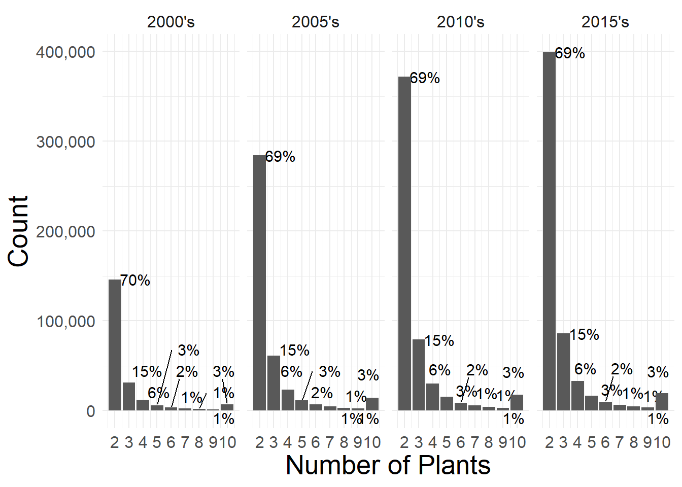
Distribution of Number of Plants per lustrum, for Multi-Plant firms

Municipal

Code

item3_municipal <- N_multi_municipal_firm_year_aff %>% 
  copy() %>% 
  # conditional on being multimunicipal; exclude non multimunicipals 
  .[N_multi_municipal_firm>1] %>% 
    # truncate at 50
    .[N_multi_municipal_firm>10, N_multi_municipal_firm := 10] %>% 
  # sum 
  .[, lustrum := paste0(2000+(floor((year-2000)/5))*5, "'s")] %>% 
  .[, sum(N), .(lustrum,N_multi_municipal_firm) ] %>% 
  .[, share := round(V1/sum(V1), digits = 2), .(lustrum) ]  
  

item3_municipal %>% 
  ggplot(., aes(x = N_multi_municipal_firm, y = V1, label = scales::percent(share, trim = F))) +
      geom_text_repel(size=2, nudge_y = 4, nudge_x = 1) +
  geom_col() + 
  facet_wrap(~lustrum) + 
    ylab("Count") +
    xlab("Number of Plants") +
    theme_minimal() +
  scale_y_continuous(labels = scales::label_comma()) + 
  scale_x_continuous(n.breaks = 10) + 
    theme(
      axis.title = element_text(size=20),
      text = element_text(size=15)
    )

  filename <- "images/distribution_n_multi_municipal_firms_lustrum.png"
  ggsave(plot = last_plot(), filename = filename, width = 16,height = 9, scale = 1)

We define a Multi-Municipal Firm as having more than one plants in different municipalities. Plants are defined by the last four digits in a firms CNPJ, excluding the last two verification digits. All firms have at least one plant by definition. The boxes in the graph indicate the yearly share of firms which are either multi-municipal or not.

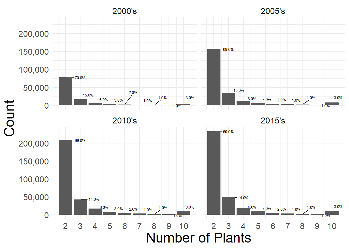
Distribution of Number of Plants per year, for Munlti-Municipal Firms

2.3.7 Number and Share of Politically Connected Firms, Conditional on being a Multi-Plants Firms

CNPJ

Code

item5_plant <- N_multi_plant_firm_year_aff %>% 
  copy() %>% 
  # conditional on being multiplant; exclude non multiplants 
  .[N_multi_plant_firm>1] %>% 
  # sum 
  .[, sum(N), .(year,firm_affiliated) ] %>% 
  .[, share := round(V1/sum(V1), digits = 3), .(year) ]  %>% 
  .[, firm_affilaited_lable := firm_affiliated==1]

item5_plant %>% 
    ggplot(., aes(x = year, y = V1, color = firm_affilaited_lable, label = scales::percent(share, trim = F))) +
    geom_label_repel(size=4) +
    geom_point() +
    geom_line() +
    ylab("Count") +
    xlab("Year") +
    labs(color = "Politically Affiliated Firm") +
    scale_y_continuous(labels = scales::label_comma()) + 
      theme_minimal() +
    theme(
      axis.title = element_text(size=25),
      legend.title = element_text(size=20),
      legend.position = "bottom",
      text = element_text(size=20)
    )

  filename <- "images/N_and_share_pc_multi_plant_firms_over_time.png"
  ggsave(plot = last_plot(), filename = filename, width = 16,height = 9, scale = 1)

We define a Multi-Plant Firm as having more than one plants in different municipalities. Plants are defined by the last four digits in a firms CNPJ, excluding the last two verification digits. All firms have at least one plant by definition. The boxes in the graph indicate the yearly share of firms which are politically connected out of all multi-plant firms in the year.

Number and Share of Politically Connected Firms, Conditional on being a Multi-Plants Firms

Municipal

Code

item5_municipal <- N_multi_municipal_firm_year_aff %>% 
  copy() %>% 
  # conditional on being multimunicipal; exclude non multimunicipals 
  .[N_multi_municipal_firm>1] %>% 
  # sum 
  .[, sum(N), .(year,firm_affiliated) ] %>% 
  .[, share := round(V1/sum(V1), digits = 3), .(year) ]  %>% 
  .[, firm_affilaited_lable := firm_affiliated==1]

item5_municipal %>% 
    ggplot(., aes(x = year, y = V1, color = firm_affilaited_lable, label = scales::percent(share, trim = F))) +
    geom_label_repel(size=4) +
    geom_point() +
    geom_line() +
    ylab("Count") +
    xlab("Year") +
    scale_y_continuous(labels = scales::label_comma()) + 

    labs(color = "Politically Affiliated Firm") +
    theme_minimal() +
    theme(
      axis.title = element_text(size=25),
      legend.title = element_text(size=20),
      legend.position = "bottom",
      text = element_text(size=20)
    )

  filename <- "images/N_and_share_pc_multi_municipal_firms_over_time.png"
  ggsave(plot = last_plot(), filename = filename, width = 16,height = 9, scale = 1)

We define a Multi-Plant Firm as having more than one plants in different municipalities. Plants are defined by the last four digits in a firms CNPJ, excluding the last two verification digits. All firms have at least one plant by definition. The boxes in the graph indicate the yearly share of firms which are politically connected out of all multi-plant firms in the year.

Number and Share of Politically Connected Firms, Conditional on being a Multi-Plants Firms

2.4 Summary Statistics

Below we present summary statistics for the data. The table caption details what was done to arrive at these statistics.

Code

quantiles <- fread("data/quantiles_table.csv") %>% 
  t() %>% 
  data.table(keep.rownames = T) 

new_names <- quantiles[1, .(V1, V2, V3, V4, V5, V6, V7)] %>% unlist() %>% append(c("variable"), .)

quantiles <- quantiles[!1] %>% 
  rename_columns(current_names = names(quantiles), new_names = new_names)

fread("data/means_table.csv") %>% 
  melt(., id.vars = c("stat")) %>%
  .[, value :=  round(value, digits =2)] %>% 
  .[, .(variable, value)] %>% 
  rename(., Mean = value) %>% 
  merge(., quantiles, "variable", all =T)

Summary Statistics

We take the pc_data data-set, restrict it to observations where firms have more than one plant per firm-year, remove all owners and keep public and private firms only.

Colonnelli, Emanuele, Valdemar Pinho Neto, and Edoardo Teso. 2022. “Politics at Work.” Working Paper 30182. Working Paper Series. National Bureau of Economic Research. https://doi.org/10.3386/w30182.

Corbi, Raphael, Elias Papaioannou, and Paolo Surico. 2018. “Regional Transfer Multipliers.” The Review of Economic Studies 86 (5): 1901–34. https://doi.org/10.1093/restud/rdy069.