Code
knitr::include_graphics("images/replication_images/figure_4_replication.png")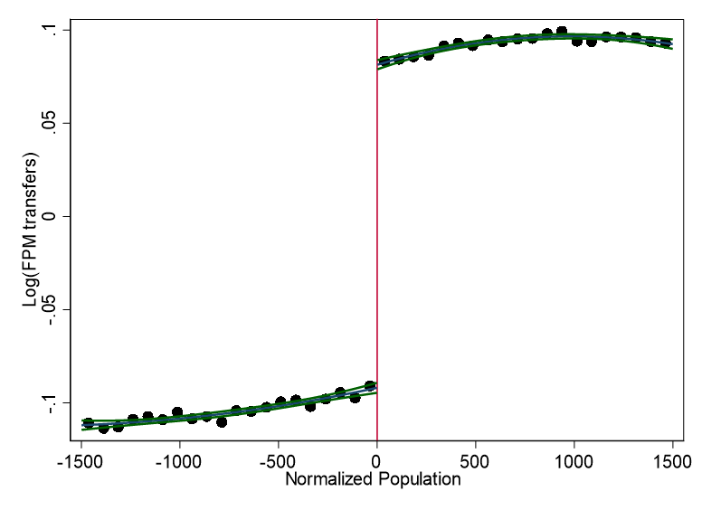
FPM transfers around the cutoffs - 2000BRL Deflators
This document was created on Monday May 29th and provides the output needed to replicate Corbi, Papaioannou, and Surico (2018) Namely, Figures 4 and 7 and table 7 from the published version of the paper.
We provide two sets of output: one for the full 2002-2019 sample and one reduced to the the common municipalities between the two data-sets.
This output was created using an adapted version of the author’s master.do file. It is split into three parts, one which does the cleaning and refers back to the master.do, and two others which create the figures and images. For more information, please see the README.txt file under ~/Dropbox/TransfersReplication/code/. All of the data is available to run their and our do files.
For an overview of the data cleaning code with some explanations behind each section, I have create an explainer available here.
knitr::include_graphics("images/replication_images/figure_4_replication.png")
FPM transfers around the cutoffs - 2000BRL Deflators
knitr::include_graphics("images/replication_images/figure_4_lfpmhat_replication.png")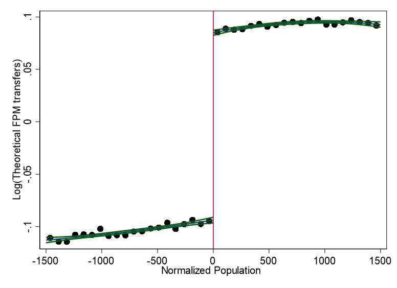
Theoretical FPM transfers around the cutoffs - 2000BRL Deflators
knitr::include_graphics("images/replication_images/figure_7a_replication.png")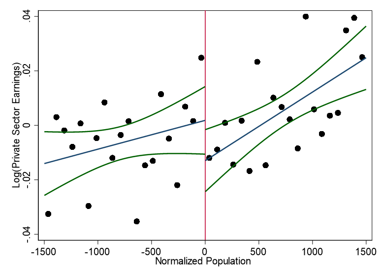
Residual log total earnings in the private sector - 2000BRL Deflators
knitr::include_graphics("images/replication_images/figure_7b_replication.png")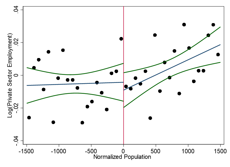
Residual log total employment in the private sector - 2000BRL Deflators
knitr::include_graphics("images/replication_images/figure_7c_replication.png")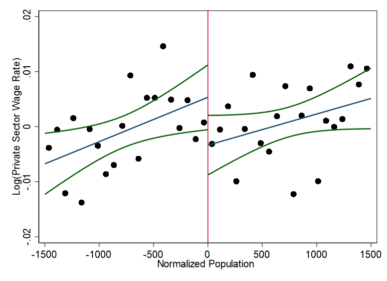
Residual log average municipality-year wages in the private sector - 2000BRL Deflators
## Clean table 7 part A

# clean the lower part of the table --------------
table7A_lower <- paste0(dir_eemt, "subprojects/transfers_replication/ouput/regression_models/xlsx/table7A_LogPrivateEmployment_replication.xlsx") %>%
  readxl::read_xlsx()  %>% as.data.table() %>% .[12:15] %>% .[, statistic := ""] %>% rename(., outcome=...1) %>%
.[, Regression := ""]


# Clean Table A; numbers -----------------
table7A_LogPrivateEmployment_replication <- paste0(dir_eemt, "subprojects/transfers_replication/ouput/regression_models/xlsx/table7A_LogPrivateEmployment_replication.xlsx") %>%
  readxl::read_xlsx()  %>% as.data.table() %>% .[3:6] %>%
  .[, ...1 := zoo::na.locf(...1)] %>% melt.data.table(id.vars = c("...1")) %>%
  .[!is.na(value)] %>%
  .[, statistic := "coefficient"] %>%
  .[stri_detect_fixed(value, "("), statistic := "se"]  %>%
  .[, outcome := "Log Private Employment"]

table7A_LogPrivateWages <- paste0(dir_eemt, "subprojects/transfers_replication/ouput/regression_models/xlsx/table7A_LogPrivateWages_replication.xlsx") %>%
  readxl::read_xlsx()   %>% as.data.table() %>% .[3:6] %>%
  .[, ...1 := zoo::na.locf(...1)] %>% melt.data.table(id.vars = c("...1")) %>%
  .[!is.na(value)] %>%
  .[, statistic := "coefficient"] %>%
  .[stri_detect_fixed(value, "("), statistic := "se"]     %>%
  .[, outcome := "Log Private Avg. Wages"]


table7A_LogPrivateEarnings <- paste0(dir_eemt, "subprojects/transfers_replication/ouput/regression_models/xlsx/table7A_LogPrivateEarnings_replication.xlsx") %>%
  readxl::read_xlsx()    %>% as.data.table() %>% .[3:6] %>%
  .[, ...1 := zoo::na.locf(...1)] %>% melt.data.table(id.vars = c("...1")) %>%
  .[!is.na(value)] %>%
  .[, statistic := "coefficient"] %>%
  .[stri_detect_fixed(value, "("), statistic := "se"]    %>%
  .[, outcome := "Log Private Total Earnings"]

table7A_main <- rbind(table7A_LogPrivateEmployment_replication, table7A_LogPrivateWages) %>%
  rbind(., table7A_LogPrivateEarnings) %>%
  dcast.data.table(formula = outcome + statistic  ~ variable, value.var = "value" ) %>%
  .[, Regression := "Reduced Form"]

# %>%    rbind(data.table(outcome=c("Reduced Form")), ., fill=T)


# Clean Table B; numbers -----------------
table7B_LogPrivateEmployment_replication <- paste0(dir_eemt, "subprojects/transfers_replication/ouput/regression_models/xlsx/table7B_LogPrivateEmployment_replication.xlsx") %>%
  readxl::read_xlsx()  %>% as.data.table() %>% .[3:4] %>%
  .[, ...1 := zoo::na.locf(...1)] %>% melt.data.table(id.vars = c("...1")) %>%
  .[!is.na(value)] %>%
  .[, statistic := "coefficient"] %>%
  .[stri_detect_fixed(value, "("), statistic := "se"]  %>%
  .[, outcome := "Log Private Employment"]

table7B_LogPrivateWages <- paste0(dir_eemt, "subprojects/transfers_replication/ouput/regression_models/xlsx/table7B_LogPrivateWages_replication.xlsx") %>%
  readxl::read_xlsx()   %>% as.data.table() %>% .[3:4] %>%
  .[, ...1 := zoo::na.locf(...1)] %>% melt.data.table(id.vars = c("...1")) %>%
  .[!is.na(value)] %>%
  .[, statistic := "coefficient"] %>%
  .[stri_detect_fixed(value, "("), statistic := "se"]     %>%
  .[, outcome := "Log Private Avg. Wages"]

table7B_LogPrivateEarnings <- paste0(dir_eemt, "subprojects/transfers_replication/ouput/regression_models/xlsx/table7B_LogPrivateEarnings_replication.xlsx") %>%
  readxl::read_xlsx()    %>% as.data.table() %>% .[3:4] %>%
  .[, ...1 := zoo::na.locf(...1)] %>% melt.data.table(id.vars = c("...1")) %>%
  .[!is.na(value)] %>%
  .[, statistic := "coefficient"] %>%
  .[stri_detect_fixed(value, "("), statistic := "se"]    %>%
  .[, outcome := "Log Private Total Earnings"]

table7B_main <- rbind(table7B_LogPrivateEmployment_replication, table7B_LogPrivateWages) %>%
  rbind(., table7B_LogPrivateEarnings) %>%
  dcast.data.table(formula = outcome + statistic  ~ variable, value.var = "value" ) %>%
  # rbind(data.table(outcome=c("IV")), ., fill=T)
  .[, Regression := "Fuzzy IV"]


table7 <- rbind(table7A_main, table7B_main, fill=T) %>%
  rbind(., table7A_lower, fill=T)


table7_present <- table7 %>% copy() %>%
  .[, outcome_hidden := outcome] %>% copy() %>%
  .[statistic=="se", outcome := ""]  %>%
    .[, statistic := NULL] %>%
.[, outcome_hidden := NULL] table7_gt<- table7_present %>%
group_by(Regression) %>%
gt() %>%
tab_spanner(
label = "Local estimates in differences",
columns = c(`(5)`, `(6)`, `(7)`, `(8)` )
) %>%
tab_spanner(
label = "Local estimates in levels",
columns = c(`(1)`, `(2)`, `(3)`, `(4)` )
) %>%
tab_spanner(
label = "<4%",
columns = c(`(1)`, `(3)`, `(5)`, `(7)` )
) %>%
tab_spanner(
label = "<2%",
columns = c(`(2)`, `(4)`, `(6)`, `(8)` )
) %>% tab_options(
column_labels.font.size = "small",
table.font.size = "small",
row_group.font.size = "small",
data_row.padding = px(3)
) %>%
sub_missing(
columns = everything(),
rows = everything(),
missing_text = "-"
)
# gtsave(table7_gt, paste0(dir_transfers_replication, "ouput/regression_models/gt_output/table7.pdf"))
table7_gt| <4% | <2% | <4% | <2% | <4% | <2% | <4% | <2% | |
|---|---|---|---|---|---|---|---|---|
| outcome | Local estimates in levels | Local estimates in differences | ||||||
| (1) | (2) | (3) | (4) | (5) | (6) | (7) | (8) | |
| Reduced Form | ||||||||
| Log Private Avg. Wages | 0.010714 | -0.015418 | -0.013432 | -0.002010 | -0.046218 | -0.065479 | -0.058503 | -0.054189 |
| (0.028) | (0.035) | (0.031) | (0.039) | (0.034) | (0.047) | (0.037) | (0.048) | |
| Log Private Employment | -0.001516 | -0.063229 | -0.015277 | -0.042993 | -0.004728 | 0.030964 | -0.021339 | 0.029839 |
| (0.055) | (0.058) | (0.063) | (0.073) | (0.044) | (0.054) | (0.053) | (0.064) | |
| Log Private Total Earnings | 0.007305 | -0.081581 | -0.029342 | -0.047140 | -0.053057 | -0.037175 | -0.084265 | -0.029728 |
| (0.059) | (0.067) | (0.069) | (0.077) | (0.053) | (0.067) | (0.057) | (0.071) | |
| Fuzzy IV | ||||||||
| Log Private Avg. Wages | 0.0115 | -0.0164 | -0.0148 | -0.00219 | - | - | - | - |
| (0.0289) | (0.0361) | (0.0331) | (0.0404) | - | - | - | - | |
| Log Private Employment | -0.00162 | -0.0674 | -0.0168 | -0.0469 | - | - | - | - |
| (0.0571) | (0.0592) | (0.0677) | (0.0768) | - | - | - | - | |
| Log Private Total Earnings | 0.00781 | -0.0869 | -0.0322 | -0.0515 | - | - | - | - |
| (0.0617) | (0.0685) | (0.0742) | (0.0803) | - | - | - | - | |
| Municipality FE | Yes | Yes | Yes | Yes | Yes | Yes | Yes | Yes |
| State-year dummies | Yes | Yes | Yes | Yes | Yes | Yes | Yes | Yes |
| Cutoff-year dummies | Yes | Yes | Yes | Yes | Yes | Yes | Yes | Yes |
| First-order polynomial | No | No | Yes | Yes | No | No | Yes | Yes |
## Clean table 7 part A
# clean the lower part of the table --------------
table7A_first_stage <- paste0(dir_eemt, "subprojects/transfers_replication/ouput/regression_models/xlsx/table7A_firststage.xlsx") %>%
  readxl::read_xlsx()  %>% as.data.table() %>%
  rename(., outcome=...1) %>% .[1:15]


# lfpm <- table7A_first_stage %>%   copy() %>%   .[3:4] %>% .[, outcome := na.locf(outcome)] %>%
#   .[, .(outcome, `(1)`, `(2)`, `(3)`, `(4)`)]
# Slfpm <- table7A_first_stage %>%   copy() %>%   .[5:6 ] %>% .[, outcome := na.locf(outcome)] %>%
# .[, .(outcome, `(5)`, `(6)`, `(7)`, `(8)`)]table7A_first_stage %>%
.[is.na(outcome), outcome := "" ] %>%
gt() %>%
sub_missing(
columns = everything(),
rows = everything(),
missing_text = "-"
) %>%
tab_spanner(
label = "Local estimates in differences",
columns = c(`(5)`, `(6)`, `(7)`, `(8)` )
) %>%
tab_spanner(
label = "Local estimates in levels",
columns = c(`(1)`, `(2)`, `(3)`, `(4)` )
) %>%
tab_spanner(
label = "<4%",
columns = c(`(1)`, `(3)`, `(5)`, `(7)` )
) %>%
tab_spanner(
label = "<2%",
columns = c(`(2)`, `(4)`, `(6)`, `(8)` )
) %>% tab_options(
column_labels.font.size = "small",
table.font.size = "small",
row_group.font.size = "small",
data_row.padding = px(3)
) Table 8.1: Table 7: First Stage
| <4% | <2% | <4% | <2% | <4% | <2% | <4% | <2% | |
|---|---|---|---|---|---|---|---|---|
| outcome | Local estimates in levels | Local estimates in differences | ||||||
| (1) | (2) | (3) | (4) | (5) | (6) | (7) | (8) | |
| VARIABLES | lfpm | lfpm | lfpm | lfpm | Slfpm | Slfpm | Slfpm | Slfpm |
| - | - | - | - | - | - | - | - | |
| lfpmhat | 0.979657*** | 0.985886*** | 0.951679*** | 0.961183*** | - | - | - | - |
| (0.005) | (0.006) | (0.006) | (0.007) | - | - | - | - | |
| Slfpmhat | - | - | - | - | 1.003015*** | 1.004928*** | 0.993876*** | 0.993824*** |
| - | - | - | - | (0.007) | (0.009) | (0.007) | (0.010) | |
| Constant | 0.304477*** | 0.210836** | 0.726752*** | 0.583636*** | 0.000764** | 0.002120*** | 0.002204*** | 0.003798*** |
| (0.072) | (0.089) | (0.087) | (0.107) | (0.000) | (0.001) | (0.001) | (0.001) | |
| - | - | - | - | - | - | - | - | |
| Observations | 12,969 | 6,171 | 12,969 | 6,171 | 9,301 | 3,617 | 9,301 | 3,617 |
| R-squared | 0.997 | 0.998 | 0.997 | 0.998 | 0.958 | 0.960 | 0.959 | 0.960 |
| Municipality FE | Yes | Yes | Yes | Yes | Yes | Yes | Yes | Yes |
| State-year dummies | Yes | Yes | Yes | Yes | Yes | Yes | Yes | Yes |
| Cutoff-year dummies | Yes | Yes | Yes | Yes | Yes | Yes | Yes | Yes |
| First-order polynomial | No | No | Yes | Yes | No | No | Yes | Yes |
?(caption)
knitr::include_graphics("images/replication_images/figure_4_replication_common.png")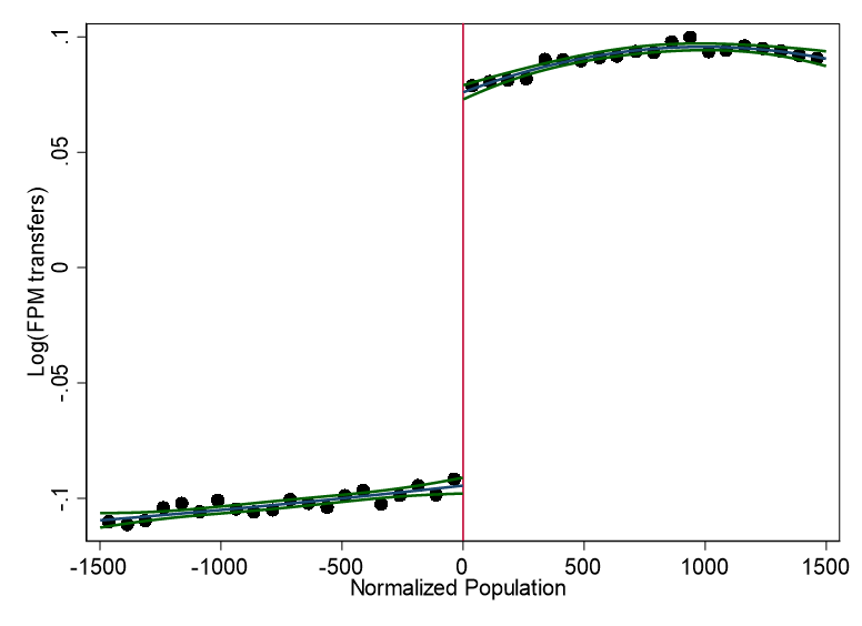
FPM transfers around the cutoffs - 2000BRL Deflators
knitr::include_graphics("images/replication_images/figure_4_lfpmhat_replication_common.png")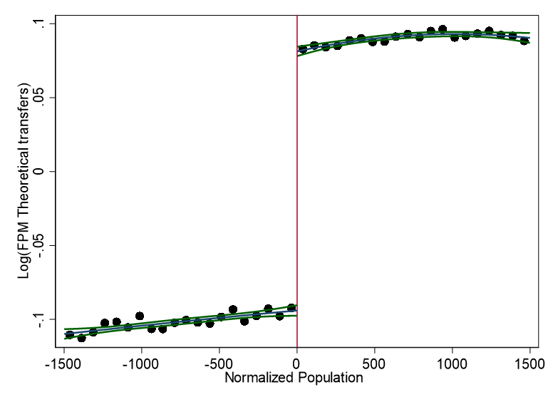
Theoretical FPM transfers around the cutoffs - 2000BRL Deflators
knitr::include_graphics("images/replication_images/figure_7a_replication_common.png")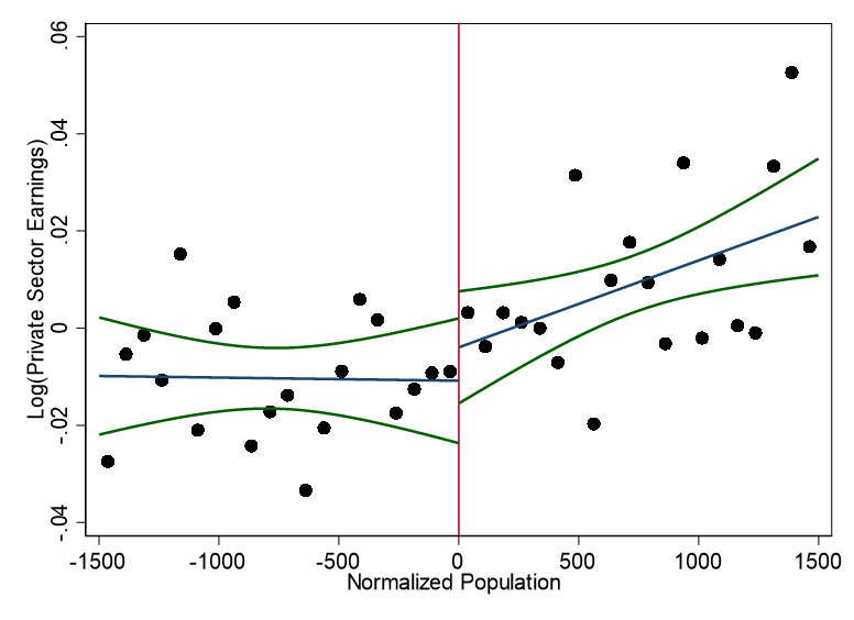
Residual log total earnings in the private sector - 2000BRL Deflators
knitr::include_graphics("images/replication_images/figure_7b_replication_common.png")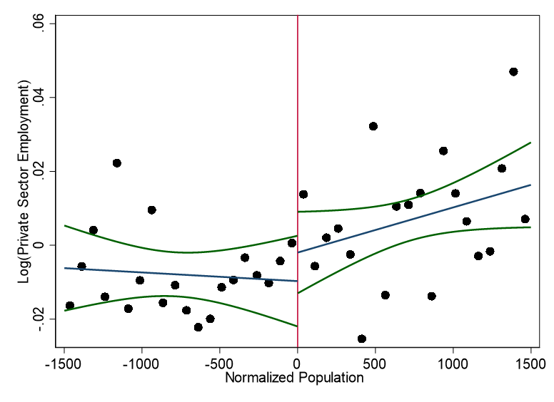
Residual log total employment in the private sector - 2000BRL Deflators
knitr::include_graphics("images/replication_images/figure_7c_replication_common.png")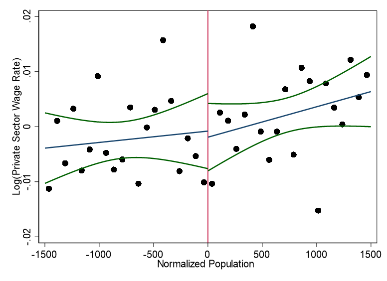
Residual log average municipality-year wages in the private sector - 2000BRL Deflators
## Clean table 7 part A

# clean the lower part of the table --------------
table7A_lower_incommon <- paste0(dir_eemt, "subprojects/transfers_replication/ouput/regression_models/xlsx/table7A_LogPrivateEmployment-InCommon_replication.xlsx") %>%
  readxl::read_xlsx()  %>% as.data.table() %>% .[10:13] %>% .[, statistic := ""] %>% rename(., outcome=...1) %>%
.[, Regression := ""]


# Clean Table A; numbers -----------------
table7A_LogPrivateEmployment2 <- paste0(dir_eemt, "subprojects/transfers_replication/ouput/regression_models/xlsx/table7A_LogPrivateEmployment-InCommon_replication.xlsx") %>%
  readxl::read_xlsx()  %>% as.data.table() %>% .[3:4] %>%
  .[, ...1 := zoo::na.locf(...1)] %>% melt.data.table(id.vars = c("...1")) %>%
  .[!is.na(value)] %>%
  .[, statistic := "coefficient"] %>%
  .[stri_detect_fixed(value, "("), statistic := "se"]  %>%
  .[, outcome := "Log Private Employment"]

table7A_LogPrivateWages2 <- paste0(dir_eemt, "subprojects/transfers_replication/ouput/regression_models/xlsx/table7A_LogPrivateWages-InCommon_replication.xlsx") %>%
  readxl::read_xlsx()   %>% as.data.table() %>% .[3:4] %>%
  .[, ...1 := zoo::na.locf(...1)] %>% melt.data.table(id.vars = c("...1")) %>%
  .[!is.na(value)] %>%
  .[, statistic := "coefficient"] %>%
  .[stri_detect_fixed(value, "("), statistic := "se"]     %>%
  .[, outcome := "Log Private Avg. Wages"]


table7A_LogPrivateEarnings2 <- paste0(dir_eemt, "subprojects/transfers_replication/ouput/regression_models/xlsx/table7A_LogPrivateEarnings-InCommon_replication.xlsx") %>%
  readxl::read_xlsx()    %>% as.data.table() %>% .[3:4] %>%
  .[, ...1 := zoo::na.locf(...1)] %>% melt.data.table(id.vars = c("...1")) %>%
  .[!is.na(value)] %>%
  .[, statistic := "coefficient"] %>%
  .[stri_detect_fixed(value, "("), statistic := "se"]    %>%
  .[, outcome := "Log Private Total Earnings"]

table7A_main_incommon <- rbind(table7A_LogPrivateEmployment2, table7A_LogPrivateWages2) %>%
  rbind(., table7A_LogPrivateEarnings2) %>%
  dcast.data.table(formula = outcome + statistic  ~ variable, value.var = "value" ) %>%
  .[, Regression := "Reduced Form"]

# %>%    rbind(data.table(outcome=c("Reduced Form")), ., fill=T)

# Clean Table B; numbers -----------------
table7B_LogPrivateEmployment2 <- paste0(dir_eemt, "subprojects/transfers_replication/ouput/regression_models/xlsx/table7B_LogPrivateEmployment-InCommon_replication.xlsx") %>%
  readxl::read_xlsx()  %>% as.data.table() %>% .[3:4] %>%
  .[, ...1 := zoo::na.locf(...1)] %>% melt.data.table(id.vars = c("...1")) %>%
  .[!is.na(value)] %>%
  .[, statistic := "coefficient"] %>%
  .[stri_detect_fixed(value, "("), statistic := "se"]  %>%
  .[, outcome := "Log Private Employment"]

table7B_LogPrivateWages2 <- paste0(dir_eemt, "subprojects/transfers_replication/ouput/regression_models/xlsx/table7B_LogPrivateWages-InCommon_replication.xlsx") %>%
  readxl::read_xlsx()   %>% as.data.table() %>% .[3:4] %>%
  .[, ...1 := zoo::na.locf(...1)] %>% melt.data.table(id.vars = c("...1")) %>%
  .[!is.na(value)] %>%
  .[, statistic := "coefficient"] %>%
  .[stri_detect_fixed(value, "("), statistic := "se"]     %>%
  .[, outcome := "Log Private Avg. Wages"]

table7B_LogPrivateEarnings2 <- paste0(dir_eemt, "subprojects/transfers_replication/ouput/regression_models/xlsx/table7B_LogPrivateEarnings-InCommon_replication.xlsx") %>%
  readxl::read_xlsx()    %>% as.data.table() %>% .[3:4] %>%
  .[, ...1 := zoo::na.locf(...1)] %>% melt.data.table(id.vars = c("...1")) %>%
  .[!is.na(value)] %>%
  .[, statistic := "coefficient"] %>%
  .[stri_detect_fixed(value, "("), statistic := "se"]    %>%
  .[, outcome := "Log Private Total Earnings"]

table7B_main_incommon <- rbind(table7B_LogPrivateEmployment2, table7B_LogPrivateWages2) %>%
  rbind(., table7B_LogPrivateEarnings2) %>%
  dcast.data.table(formula = outcome + statistic  ~ variable, value.var = "value" ) %>%
  # rbind(data.table(outcome=c("IV")), ., fill=T)
  .[, Regression := "Fuzzy IV"]

table7_incommon <- rbind(table7A_main_incommon, table7B_main_incommon, fill=T) %>%
  rbind(., table7A_lower_incommon, fill=T)

table7_incommon_present <- table7_incommon %>% copy() %>%
  .[, outcome_hidden := outcome] %>% copy() %>%
  .[statistic=="se", outcome := ""]  %>%
    .[, statistic := NULL] %>%
.[, outcome_hidden := NULL] table7_incommon_gt <- table7_incommon_present %>%
group_by(Regression) %>%
gt() %>%
tab_spanner(
label = "Local estimates in levels",
columns = c(`(1)`, `(2)`, `(3)`, `(4)` )
) %>%
tab_spanner(
label = "<4%",
columns = c(`(1)`, `(3)` )
) %>%
tab_spanner(
label = "<2%",
columns = c(`(2)`, `(4)` )
) %>% tab_options(
column_labels.font.size = "small",
table.font.size = "small",
row_group.font.size = "small",
data_row.padding = px(3)
) %>%
sub_missing(
columns = everything(),
rows = everything(),
missing_text = "-"
)
# gtsave(table7_incommon_gt, paste0(dir_transfers_replication, "ouput/regression_models/gt_output/table7_incommon.pdf"))
table7_incommon_gt| <4% | <2% | <4% | <2% | |
|---|---|---|---|---|
| outcome | Local estimates in levels | |||
| (1) | (2) | (3) | (4) | |
| Reduced Form | ||||
| Log Private Avg. Wages | 0.061591** | 0.050169 | 0.033099 | 0.044230 |
| (0.031) | (0.043) | (0.034) | (0.051) | |
| Log Private Employment | 0.003198 | -0.026708 | 0.019555 | 0.010105 |
| (0.057) | (0.071) | (0.065) | (0.085) | |
| Log Private Total Earnings | 0.066876 | 0.023298 | 0.056161 | 0.054546 |
| (0.060) | (0.082) | (0.066) | (0.096) | |
| Fuzzy IV | ||||
| Log Private Avg. Wages | 0.0656** | 0.0529 | 0.0363 | 0.0479 |
| (0.0318) | (0.0428) | (0.0362) | (0.0523) | |
| Log Private Employment | 0.00341 | -0.0281 | 0.0215 | 0.0109 |
| (0.0597) | (0.0708) | (0.0693) | (0.0871) | |
| Log Private Total Earnings | 0.0712 | 0.0245 | 0.0617 | 0.0590 |
| (0.0623) | (0.0820) | (0.0712) | (0.0990) | |
| Municipality FE | Yes | Yes | Yes | Yes |
| State-year dummies | Yes | Yes | Yes | Yes |
| Cutoff-year dummies | Yes | Yes | Yes | Yes |
| First-order polynomial | No | No | Yes | Yes |
This table replicates the output from table 7 using the intersection of the municipalities in our data and theirs, between 2002-2014.
## Clean table 7 part A

"C:/Users/alckm/Dropbox/EEMT/subprojects/transfers_replication/ouput/regression_models/xlsx/table7A_firststage_incommon.xlsx"
[1] "C:/Users/alckm/Dropbox/EEMT/subprojects/transfers_replication/ouput/regression_models/xlsx/table7A_firststage_incommon.xlsx"# clean the lower part of the table --------------
table7A_first_stage_common <- paste0(dir_eemt, "subprojects/transfers_replication/ouput/regression_models/xlsx/table7A_firststage_incommon.xlsx") %>%
readxl::read_xlsx() %>% as.data.table() %>%
rename(., outcome=...1) %>% .[1:15]
# lfpm <- table7A_first_stage %>% copy() %>% .[3:4] %>% .[, outcome := na.locf(outcome)] %>%
# .[, .(outcome, `(1)`, `(2)`, `(3)`, `(4)`)]
# Slfpm <- table7A_first_stage %>% copy() %>% .[5:6 ] %>% .[, outcome := na.locf(outcome)] %>%
# .[, .(outcome, `(5)`, `(6)`, `(7)`, `(8)`)]table7A_first_stage_common %>%
.[is.na(outcome), outcome := "" ] %>%
gt() %>%
sub_missing(
columns = everything(),
rows = everything(),
missing_text = "-"
) %>%
tab_spanner(
label = "Local estimates in differences",
columns = c(`(5)`, `(6)`, `(7)`, `(8)` )
) %>%
tab_spanner(
label = "Local estimates in levels",
columns = c(`(1)`, `(2)`, `(3)`, `(4)` )
) %>%
tab_spanner(
label = "<4%",
columns = c(`(1)`, `(3)`, `(5)`, `(7)` )
) %>%
tab_spanner(
label = "<2%",
columns = c(`(2)`, `(4)`, `(6)`, `(8)` )
) %>% tab_options(
column_labels.font.size = "small",
table.font.size = "small",
row_group.font.size = "small",
data_row.padding = px(3)
) Table 8.3: Table 7: First Stage
| <4% | <2% | <4% | <2% | <4% | <2% | <4% | <2% | |
|---|---|---|---|---|---|---|---|---|
| outcome | Local estimates in levels | Local estimates in differences | ||||||
| (1) | (2) | (3) | (4) | (5) | (6) | (7) | (8) | |
| VARIABLES | lfpm | lfpm | lfpm | lfpm | Slfpm | Slfpm | Slfpm | Slfpm |
| - | - | - | - | - | - | - | - | |
| lfpmhat | 0.992804*** | 1.001072*** | 0.960541*** | 0.972053*** | - | - | - | - |
| (0.006) | (0.007) | (0.007) | (0.009) | - | - | - | - | |
| Slfpmhat | - | - | - | - | 1.018091*** | 1.032847*** | 1.008031*** | 1.018742*** |
| - | - | - | - | (0.008) | (0.010) | (0.008) | (0.012) | |
| Constant | 0.104443 | -0.020119 | 0.589723*** | 0.416474*** | -0.000339 | 0.000363 | 0.001393 | 0.002212 |
| (0.088) | (0.112) | (0.107) | (0.131) | (0.000) | (0.001) | (0.001) | (0.001) | |
| - | - | - | - | - | - | - | - | |
| Observations | 9,079 | 4,202 | 9,079 | 4,202 | 6,141 | 2,310 | 6,141 | 2,310 |
| R-squared | 0.997 | 0.998 | 0.997 | 0.998 | 0.961 | 0.963 | 0.961 | 0.964 |
| Municipality FE | Yes | Yes | Yes | Yes | Yes | Yes | Yes | Yes |
| State-year dummies | Yes | Yes | Yes | Yes | Yes | Yes | Yes | Yes |
| Cutoff-year dummies | Yes | Yes | Yes | Yes | Yes | Yes | Yes | Yes |
| First-order polynomial | No | No | Yes | Yes | No | No | Yes | Yes |
?(caption)